
Syllabus
Assumed knowledge (from year 11 Mathematics Specialist content)
This content will be only briefly reviewed as part of the year 12 course.
Representing vectors in the plane by directed line segments
1.2.1 examine examples of vectors, including displacement and velocity
1.2.2 define and use the magnitude and direction of a vector
1.2.3 represent a scalar multiple of a vector
1.2.4 use the triangle and parallelogram rules to find the sum and difference of two vectors
Algebra of vectors in the plane
1.2.5 use ordered pair notation and column vector notation to represent a vector
1.2.6 define unit vectors and the perpendicular unit vectors i and j
1.2.7 express a vector in component form using the unit vectors i and j
1.2.8 examine and use addition and subtraction of vectors in component form
1.2.9 define and use multiplication of a vector by a scalar in component form
1.2.10 define and use scalar (dot) product
1.2.11 apply the scalar product to vectors expressed in component form
1.2.12 examine properties of parallel and perpendicular vectors and determine if two vectors are parallel or perpendicular
1.2.13 define and use projection of vectors
1.2.14 solve problems involving displacement, force and velocity involving the above concepts
Topic 3.3: Vectors in three dimensions (21 hours)
The algebra of vectors in three dimensions
3.3.1 review the concepts of vectors from Unit 1 and extend to three dimensions, including introducing the unit vectors i, j and k
3.3.2 prove geometric results in the plane and construct simple proofs in 3 dimensions
Vector and Cartesian equations
3.3.3 introduce Cartesian coordinates for three dimensional space, including plotting points and equations of spheres
3.3.4 use vector equations of curves in two or three dimensions involving a parameter and determine a ‘corresponding’ Cartesian equation in the two-dimensional case
3.3.5 determine a vector equation of a straight line and straight line segment, given the position of two points or equivalent information, in both two and three dimensions
3.3.6 examine the position of two particles, each described as a vector function of time, and determine if their paths cross or if the particles meet
3.3.7 use the cross product to determine a vector normal to a given plane
3.3.8 determine vector and Cartesian equations of a plane
Systems of linear equations
3.3.9 recognise the general form of a system of linear equations in several variables, and use elementary techniques of elimination to solve a system of linear equations
3.3.10 examine the three cases for solutions of systems of equations – a unique solution, no solution, and infinitely many solutions – and the geometric interpretation of a solution of a system of equations with three variables
Vector calculus
3.3.11 consider position vectors as a function of time
3.3.12 derive the Cartesian equation of a path given as a vector equation in two dimensions, including ellipses and hyperbolas
3.3.13 differentiate and integrate a vector function with respect to time
3.3.14 determine equations of motion of a particle travelling in a straight line with both constant and variable acceleration
3.3.15 apply vector calculus to motion in a plane, including projectile and circular motion
Lessons
1. Extending from two dimensions to three dimensions
2. Vector equation of a line
3. Vector and Cartesian Equations; Parametric Equations
4. Vector Equation of a Plane (including normal/dot product form for equations of lines in 2D and planes in 3D, and including cross product.)
5. Sample applications: Collision, Closest Approach and Interception
Determining whether paths cross or if particles intercept each other is clearly part of the syllabus. Interception and Closest Approach problems are extensions of these ideas that may be encountered even though they are not explicitly mentioned in the syllabus.
https://prezi.com/view/68ixiaZlhnYE3H5MrgOa/
Prezi: Vector Applications
6. Vector Proof
Vectors provide a method that simplifies proof of a number of geometric theorems.
Some general principles:
- Select key intervals and set a vector equal to each, then express other intervals in terms of those vectors. For example, if working with a parallelogram ABCD, you should make vector b equal to interval AB, and vector d equal to interval AD. Interval AC, then, is equal to b+d, etc.
- Do not use more vectors than you need. Most (but not all) 2D proofs will only need two vectors. Most 3D proofs will only need three vectors. If you have already introduced vectors a and b, don’t introduce a third vector c if it can be written in terms of a and b instead.
Example: Prove that the diagonals of a kite are perpendicular.
Step 1. Draw a diagram. Try to avoid special cases (like lines at right angles, or lines the same length, or equal angles) that are not specified in the proposition. Show the information that is given. Here, we know it’s a kite so we should show two pairs of adjacent sides the same length. (We could also show one pair of opposite angles equal, but angles other than right angles aren’t used so often in vector proofs.)
Step 2. Label the diagram. It is often useful to choose a key point to treat as the origin, and label it O.
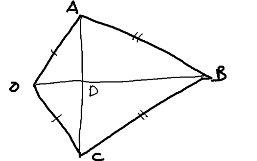
Step 3. Rewrite the proposition in terms of the diagram: required to prove: OB is perpendicular to AC.
Step 4. Set up vectors. Here we need three: Let 


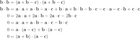
Step 5. Write down other key vectors in terms of these. Here the key vectors are 


Step 6. Think about what the proposition means in vector terms. If 
Step 7. Think about what else we know, in vector terms. Here we know that the lengths of OA and OC are equal, so 


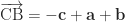


Step 8. Manipulate these to result in the proposition:
7. Vector Calculus
See https://youtu.be/Q8b9r7forJA for a nice example of vector calculus used to derive the formula for centripetal acceleration.
8. Systems of Linear Equations
This is introduced as a series of four short videos:
As a follow-up, what happens if we try to find the equation of the line that is the solution to the last example? This document explores that further: simult6.
This Prezi looks at the geometric interpretation of the various situations when solving simultaneous equations in two and three dimensions. (TODO: this Prezi has no narration.)
Other resources that may be helpful:
- https://www.khanacademy.org/math/precalculus/precalc-matrices/representing-systems-with-matrices/a/representing-systems-with-matrices. This link is definitely relevant and may be worthwhile if you’re still trying to get your head around using matrices for systems of equations.
- https://www.khanacademy.org/math/linear-algebra/vectors_and_spaces/matrices_elimination/v/matrices-reduced-row-echelon-form-1. This is a more advanced video and sets what we are doing here in the broader context of the mathematical topic of linear algebra. It may go beyond what we’re doing and it may use language that you’re unfamiliar with.
Exercises
See the Topics in Secondary Mathematics: Matrices section 2.1 page 25. Relevant questions include 1 — 28. (It may also be useful to revise row operations and do a selection of exercises from section 1.5, page 9ff. Questions 45 — 64 should be achievable.)
Incidental content
An interesting way of deriving the sine and cosine laws of triangles from vector and scalar products can be found in this document: sine-cosine-laws.
