Syllabus

Topic 4.1: Integration and applications of integration (20 hours)

Integration techniques

4.1.1 integrate using the trigonometric identities $\sin^2x=\frac12(1-\cos2x)$ , $\cos^2x=\frac12(1+\cos2x)$ and $1+\tan^2x=sec^2x$

4.1.2 use substitution $u=g(x)$ to integrate expressions of the form $f(g(x))g'(x)$

4.1.3 establish and use the formula $\int\frac1xdx=\ln|x|+c\text{ for }x\neq0$

4.1.4 use partial fractions where necessary for integration in simple cases

Applications of integral calculus

4.1.5 calculate areas between curves determined by functions

4.1.6 determine volumes of solids of revolution about either axis

4.1.7 use technology with numerical integration

Lessons

For other work on Integration techniques, refer to notes on SEQTA and class work.

1. Integration by Change of Variable (u-Substitution)

https://prezi.com/mb-npczyhr4j/?utm_campaign=share&utm_medium=copy&rc=ex0share

Integration by change of variable

See the document below for worked solutions to the trig substitution questions in the Prezi.

trig-substitution-solutions Download

2. Integrating Powers of Trig Functions

https://prezi.com/kcxurikmlfyq/?utm_campaign=share&utm_medium=copy&rc=ex0share

Integrating powers of trig functions

3. Area Under and Between Curves

You should already be familiar with area under curve calculations. This extends that idea to area between curves. The Prezi starts with area under a curve and then builds on those ideas for area between curves.
The video covers only area under a curve, and covers it in a different way from the Prezi. You should treat it as revision of prior work with integration.

Area under a curve from Glen Prideaux on Vimeo.

See interactive diagrams showing area under a curve or area between curves.

4. Solids of Revolution

This is not something that I have prepared a Prezi for so I will be using Khan Academy for the principal reference. See the videos and exercises at https://www.khanacademy.org/math/integral-calculus/solid-revolution-topic/disc-method/e/volumes-of-solids-of-revolution–discs-and-washers. Students should view at least the first two or three videos then work through the exercises at the end of this section of videos at least twice, viewing other videos as they encounter the need. Next, move on to the Shell Method at https://www.khanacademy.org/math/integral-calculus/solid-revolution-topic/shell-method/v/shell-method-for-rotating-around-vertical-line, viewing at least two of the videos there then working through the exercises a couple of times. (The shell method is more obscure and not as important as the disc method. Many situations that are suitable for the shell method can be done by the disc method instead. You should be familiar with the shell method, but you should practice the disc method until you can do it about either axis in your sleep.)

Another useful resource is Eddie Woo’s fine videos on this topic at https://youtu.be/XUoNadN2SbE, https://youtu.be/0BQiIF8wca8, https://youtu.be/fjsNIw1tLl4, https://youtu.be/_1GtrOWyif8.

5. Numerical Integration

1. Calculating a Riemann Sum in a spreadsheet
First, review Riemann Sums: https://www.khanacademy.org/math/integral-calculus/indefinite-definite-integrals/riemann-sums/v/simple-riemann-approximation-using-rectangles
2. Examine different approaches that converge faster than a Riemann Sum

The trapezium rule: models each slice using a trapezium. For n slices,
$\displaystyle\int_a^b f(x)\,dx\approx\sum_{i=1}^n\left(\frac{f(x_{i-1})+f(x_i)}2\times w\right)$
where $w=\frac{b-a}n$ and $x_i=a+iw$ . This simplifies to
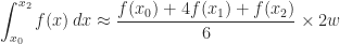
$\displaystyle \int_a^b f(x),dx\approx w \left(\frac{f(a)+f(b)}2+\sum_{i=1}^{n-1} f(x_i)\right)$
(Can you demonstrate the simplification?)
Simpson’s Rule: this converges faster than simpler rules. It approximates the area of each slice by using a quadratic approximation of the curve. For Simpson’s rule, each slice is defined by two end points and a mid point, and the area of a single slice of width $2w$ is given by
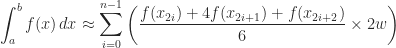
$\displaystyle \int_{x_0}^{x_2} f(x)\,dx\approx \frac{f(x_0)+4f(x_1)+f(x_2)}{6}\times 2w$
(where $x_1=x_0+w=x_2-w$ ). For n slices of width 2w then the sum becomes
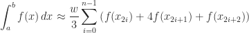
$\displaystyle \int_{a}^{b} f(x)\,dx\approx \sum_{i=0}^{n-1}\left(\frac{f(x_{2i})+4f(x_{2i+1})+f(x_{2i+2})}{6}\times 2w\right)$
which simplifies to
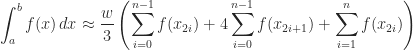
$\displaystyle \int_{a}^{b} f(x)\,dx\approx \frac{w}{3}\sum_{i=0}^{n-1}\left(f(x_{2i})+4f(x_{2i+1})+f(x_{2i+2})\right)$
then splitting the sum
$\displaystyle\int_{a}^{b} f(x)\,dx\approx \frac{w}{3}\left(\sum_{i=0}^{n-1}f(x_{2i})+4\sum_{i=0}^{n-1}f(x_{2i+1})+\sum_{i=0}^{n-1}f(x_{2i+2})\right)$
tweaking the third sum gives
$\displaystyle \int_{a}^{b} f(x)\,dx\approx \frac{w}{3}\left(\sum_{i=0}^{n-1}f(x_{2i})+4\sum_{i=0}^{n-1}f(x_{2i+1})+\sum_{i=1}^{n}f(x_{2i})\right)$
Now the third sum and the first sum are identical except for the $f(x_0)=f(a)$ term included only in the first term, and the $f(x_{2n})=f(b)$ included only in the last term. This gives us
$\displaystyle\int_{a}^{b} f(x)\,dx\approx \frac{w}{3}\left(f(a)+f(b)+2\sum_{i=1}^{n-1}f(x_{2i})+4\sum_{i=0}^{n-1}f(x_{2i+1})\right)$
Remember, here $w$ is only half the width of each slice, so $w=\frac{b-a}{2n}$ but $x_i=a+iw$ as previously.